Plot feature contribution as a bar graph

Plot previously calculated feature contribution as a bar graph.

lgb.plot.interpretation(tree_interpretation_dt, top_n = 10, cols = 1,
  left_margin = 10, cex = NULL)

Arguments

tree_interpretation_dt	a data.table returned by lgb.interprete.
top_n	maximal number of top features to include into the plot.
cols	the column numbers of layout, will be used only for multiclass classification feature contribution.
left_margin	(base R barplot) allows to adjust the left margin size to fit feature names.
cex	(base R barplot) passed as cex.names parameter to barplot.

Value

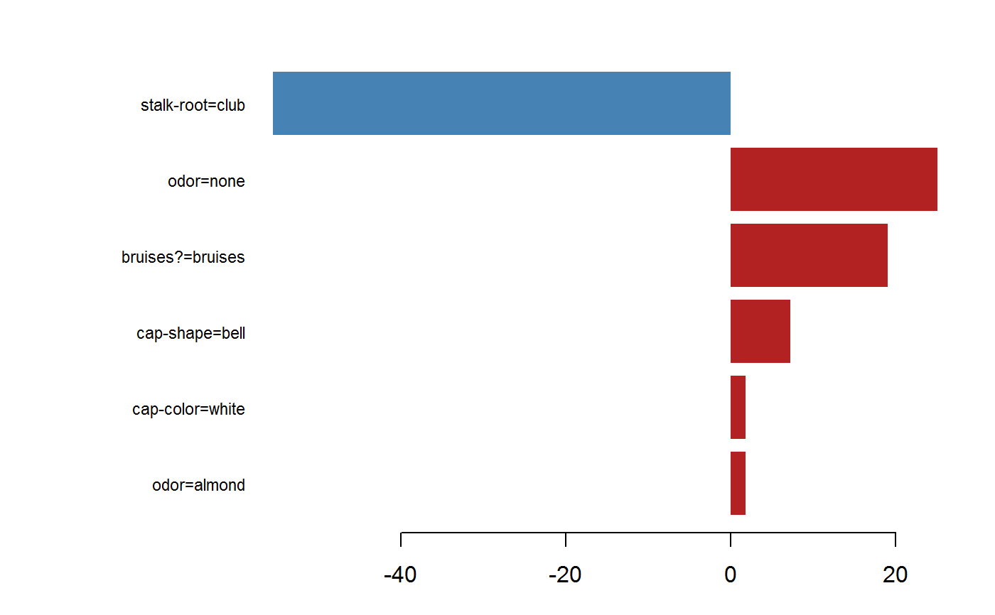
The lgb.plot.interpretation function creates a barplot.

Details

The graph represents each feature as a horizontal bar of length proportional to the defined contribution of a feature. Features are shown ranked in a decreasing contribution order.

Examples

library(lightgbm)
Sigmoid <- function(x) {1 / (1 + exp(-x))}
Logit <- function(x) {log(x / (1 - x))}
data(agaricus.train, package = "lightgbm")
train <- agaricus.train
dtrain <- lgb.Dataset(train$data, label = train$label)
setinfo(dtrain, "init_score", rep(Logit(mean(train$label)), length(train$label)))
data(agaricus.test, package = "lightgbm")
test <- agaricus.test

params <- list(objective = "binary",
              learning_rate = 0.01, num_leaves = 63, max_depth = -1,
              min_data_in_leaf = 1, min_sum_hessian_in_leaf = 1)
              model <- lgb.train(params, dtrain, 20)
model <- lgb.train(params, dtrain, 20)

tree_interpretation <- lgb.interprete(model, test$data, 1:5)
lgb.plot.interpretation(tree_interpretation[[1]], top_n = 10)